Teaching with NYC Open Data: Publishing Student Civic Research Through Reproducible Workflows
Teaching with NYC Open Data
Christian A. Martinez
Brooklyn College, City University of New York (CUNY)
NYC Open Data Week 2026
Resources
Why This Matters
I realized my students were learning to “juggle upside down.”
They weren’t struggling with the code—
they were struggling with the relevance.
The Shift
- Replace generic datasets with NYC Open Data
- Let students study their own neighborhoods, systems, and experiences
The Result
👉 Learning actually sticks
Crystal Adote
NYC Leading Causes of Death and Environmental Complaints
Overview
My project examines the leading causes of death in NYC from 2007–2014, and indoor environmental complaints such as mold, indoor air quality, asbestos, and more from 2010 to the present. I wanted to explore these datasets and see whether there were any relationships between the two.
Indoor Environmental Complaint Types
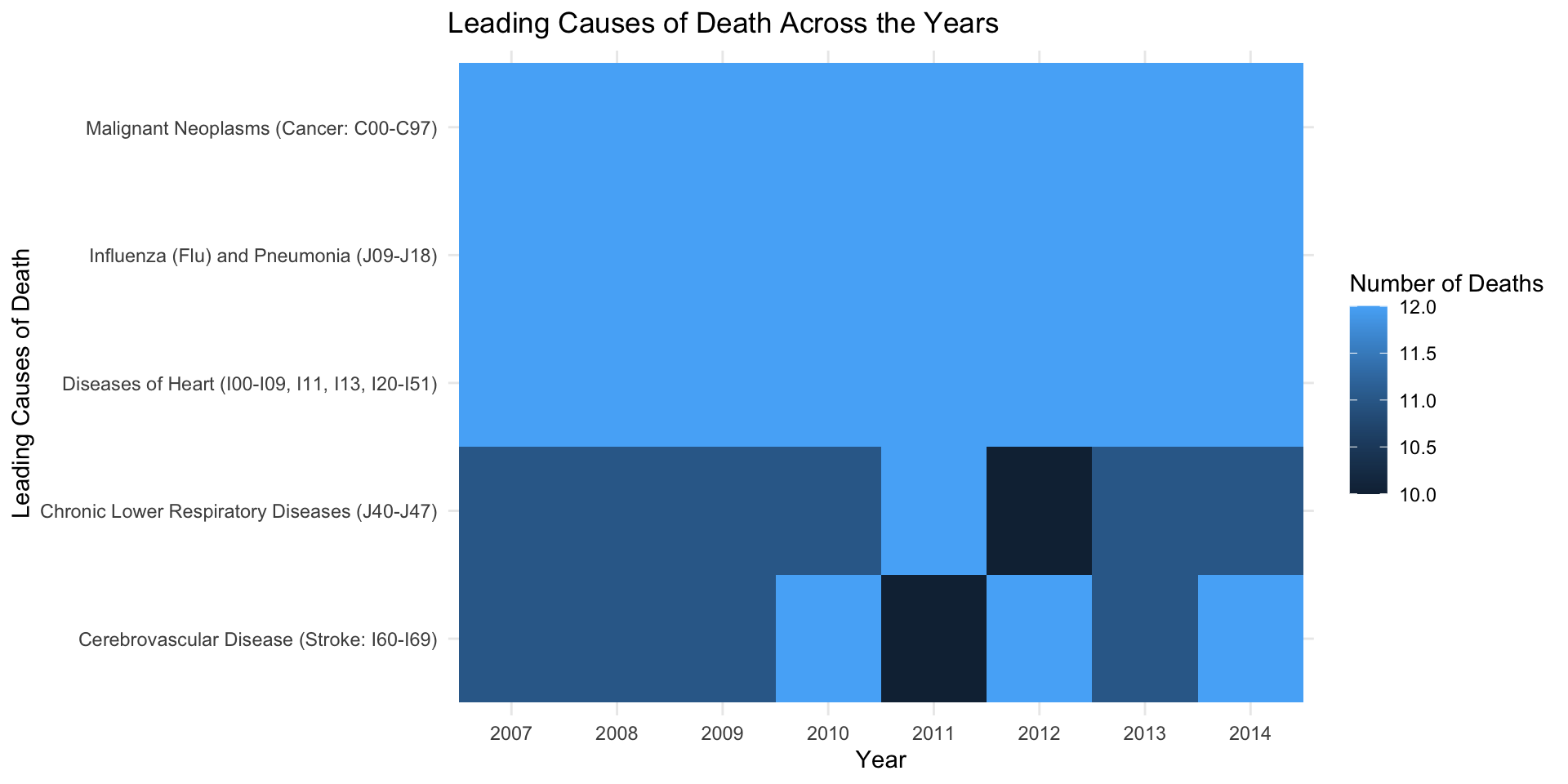
![This is a Heatmap that conveys 5 of the leading causes of death over the years]()
Figure 1: This is a Heatmap that conveys 5 of the leading causes of death over the years
Leading Causes of Death
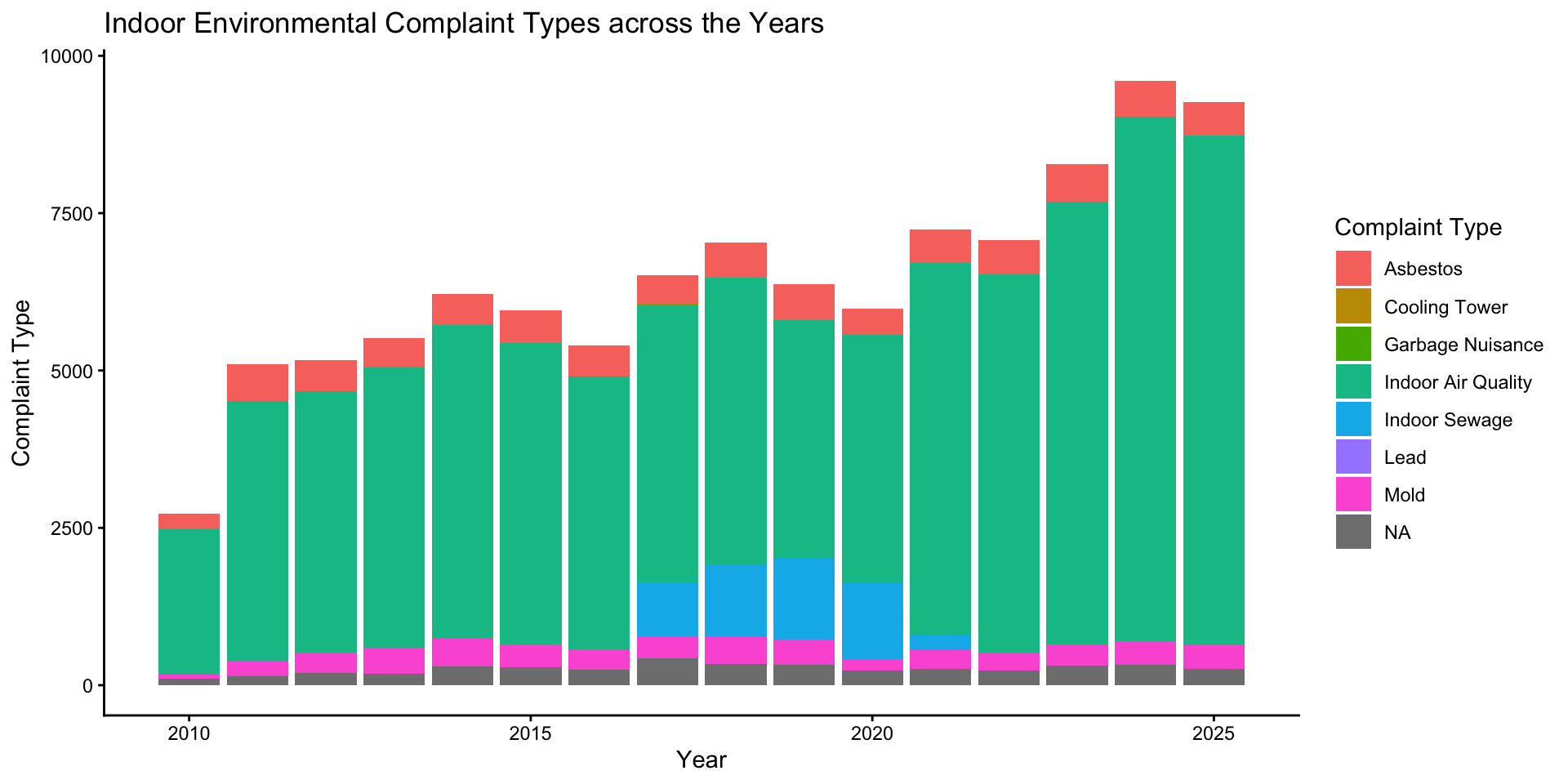
![This stacked bar graph conveys the amount of indoor environmental complaints over the years]()
Figure 2: This stacked bar graph conveys the amount of indoor environmental complaints over the years
Data Cleaning and Analysis
- Took out columns that were not needed
- Kept only five common, well-known causes of death
- Paired complaint types with causes of death
- Merged the two datasets
Statistical Tests
- Correlation: r = 0.6122905
- Linear regression suggested that indoor complaint types did not show a meaningful relationship with the leading causes of death in NYC.
Takeaway
- This topic is important to the general community because it sheds light on indoor environmental hazards that individuals file complaints about.
- It also raises questions about whether there may be a relationship between indoor environmental hazards and leading causes of death in NYC.
Jonah Dratfield
Social Infrastructure & Well-being
The Overarching Questions
Can publicly available data be used to explore the conditions that best facilitate social connectedness, and thereby, most enhance quality of life?
Is there already data that points to “abstract” psychological constructs like well-being, loneliness, etc?
If so, is how can this data be acted upon or improved?
Some (Partial) Answers
At present, NYC Open Data does not include the validated measures psychologists typically use to assess metrics like social connectedness and well-being.
However, there are various proxies.
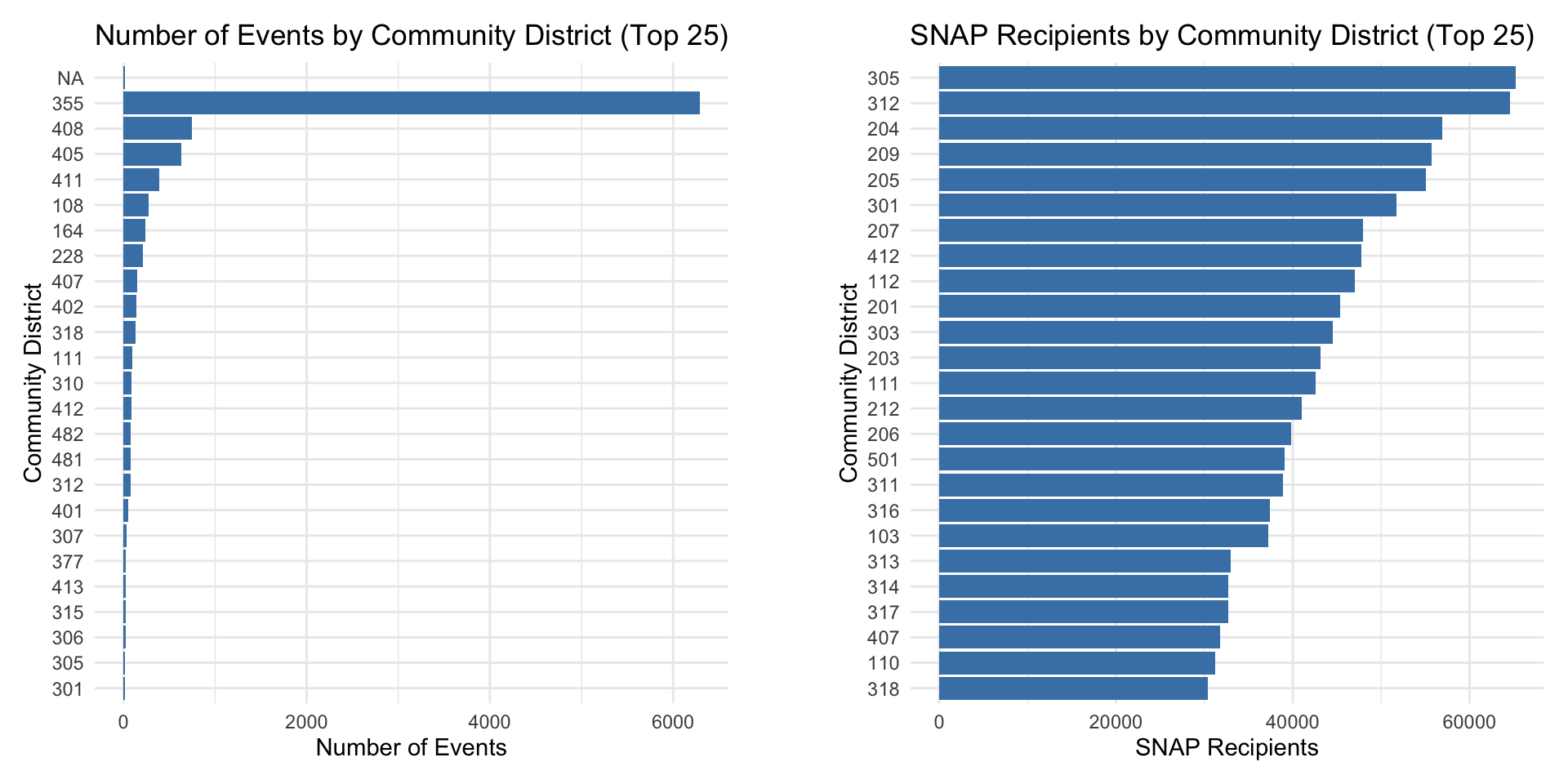
Permitted events are a proxy for connectedness.
Number of SNAP Benefit Recipients is a (very) rough proxy for economic health (which is often associated with well-being).
Results
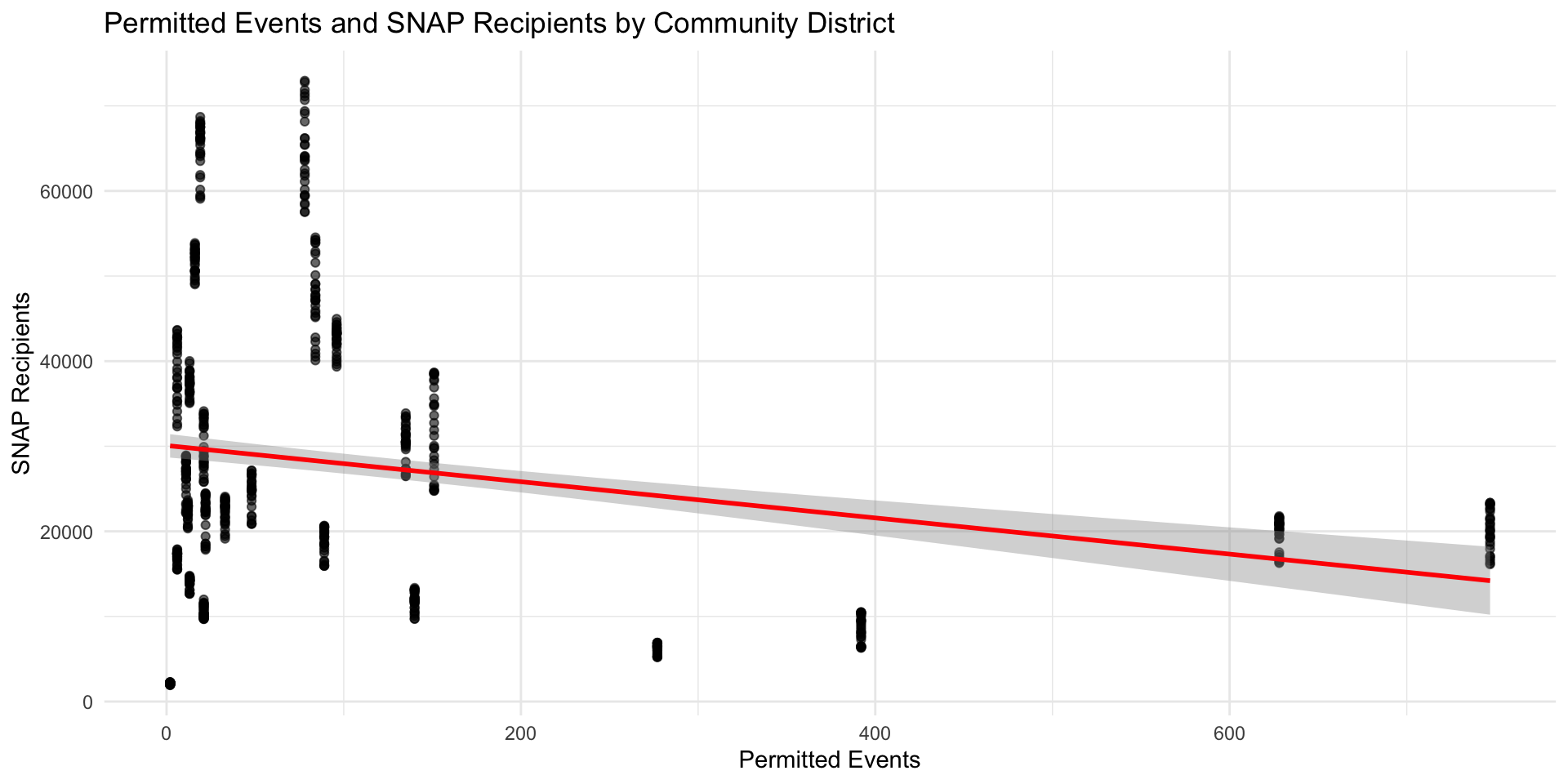
A linear regression was conducted to determine whether number of permitted events predicts number of SNAP recipients.
The model was statistically significant, F(1, 723) = 45.34, p < .001, and explained approximately 6% of the variance in SNAP recipients (R² = .059).
The number of events was a significant negative predictor of SNAP recipients, b = −21.30, SE = 3.16, t(723) = −6.73, p < .001.
Permitted Events/SNAP Linear Model
![]()
Figure 4
Limitations
Results are significant and promising … but …
SNAP is an imperfect measure of holistic well-being (as well as economic). We need more “middle range” data.
We need better social gathering info (Reddit, Meetup, Eventbrite, etc.)
Community districts are imperfect units. Access is as important as location. Parks, for instance, were excluded from the analysis.
Joyce Escatel-Flores
NYC Art Meets NYC Appetite
Goals of the Project
Explore whether restaurants near art museums are more likely to have higher ratings than restaurants not close to museums.
Explore whether restaurants near museums are less likely to have no violation citations than restaurants not close to museums.
Creating an interactive map that pinpoints restaurants that are nearby museums.
Data Sets Used
- DOHMH New York City Restaurant Inspection results which you can find at https://data.cityofnewyork.us/Health/DOHMH-New-York-City-Restaurant-Inspection-Results/43nn-pn8j/about_data
- MUSEUM which you can find at https://data.cityofnewyork.us/Recreation/MUSEUM/fn6f-htvy/about_data
The third data set is a Kaggle open data set created by Beridzeg45 called NYC Restaurants, which you can find at https://www.kaggle.com/datasets/beridzeg45/nyc-restaurants
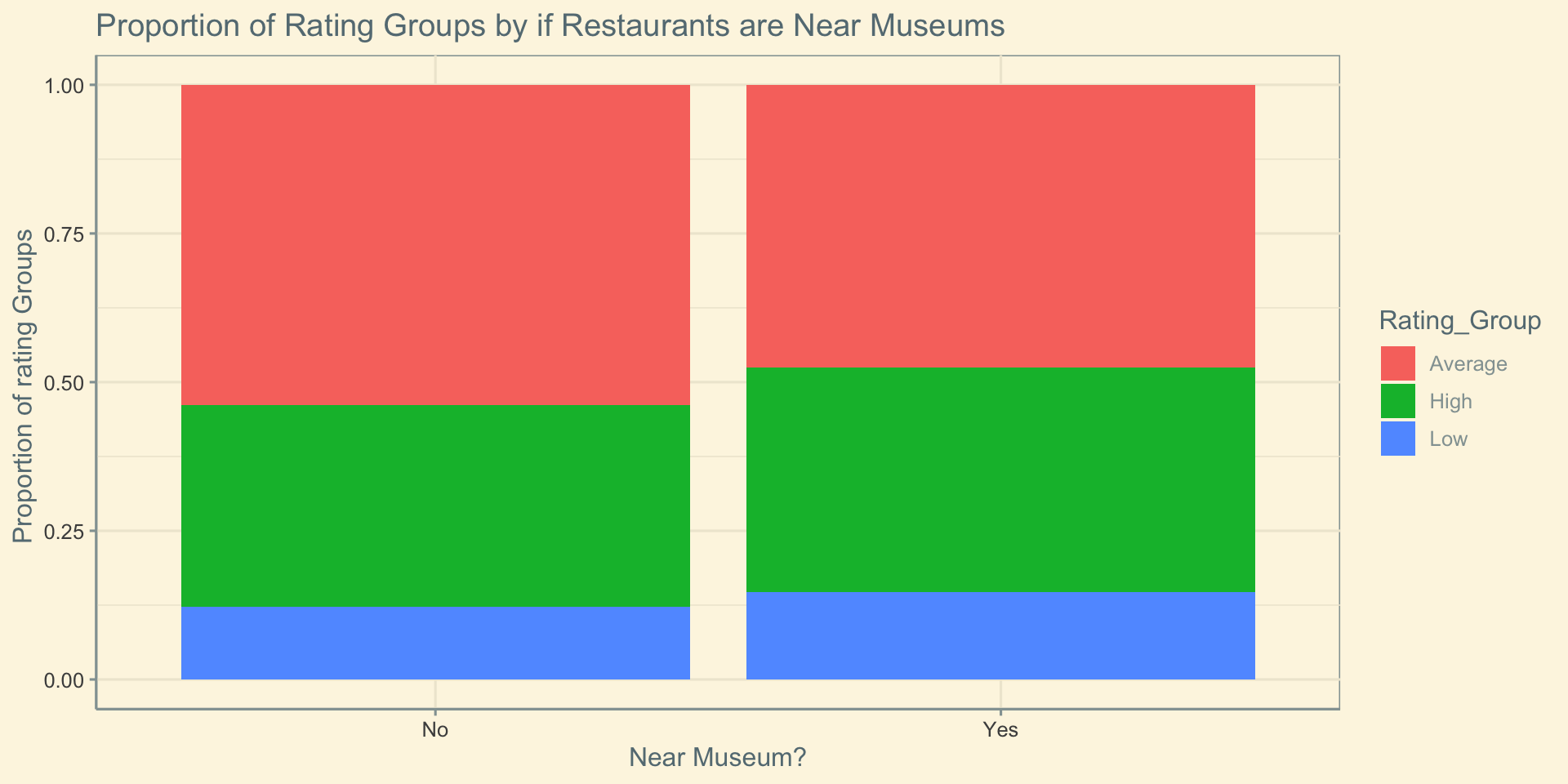
Goal 1: Visualizing the Analysis
We are visualizing the proportion of rating groups (high, medium, low) by if restaurants are near museums (yes,no).
![]()
Figure 5
Chi-Square Analysis for Goal 1
    Pearson's Chi-squared test

data:  contingency_table
X-squared = 1.1849, df = 2, p-value = 0.553
The chi-square test shows X^2 = 0.64691 (0.65), df = 2, p = 0.7236 (0.72)
There is not a statistically significant relationship between restaurants being near museums and rating.
Cramer’s V tells us that the relationship is weak in strength.
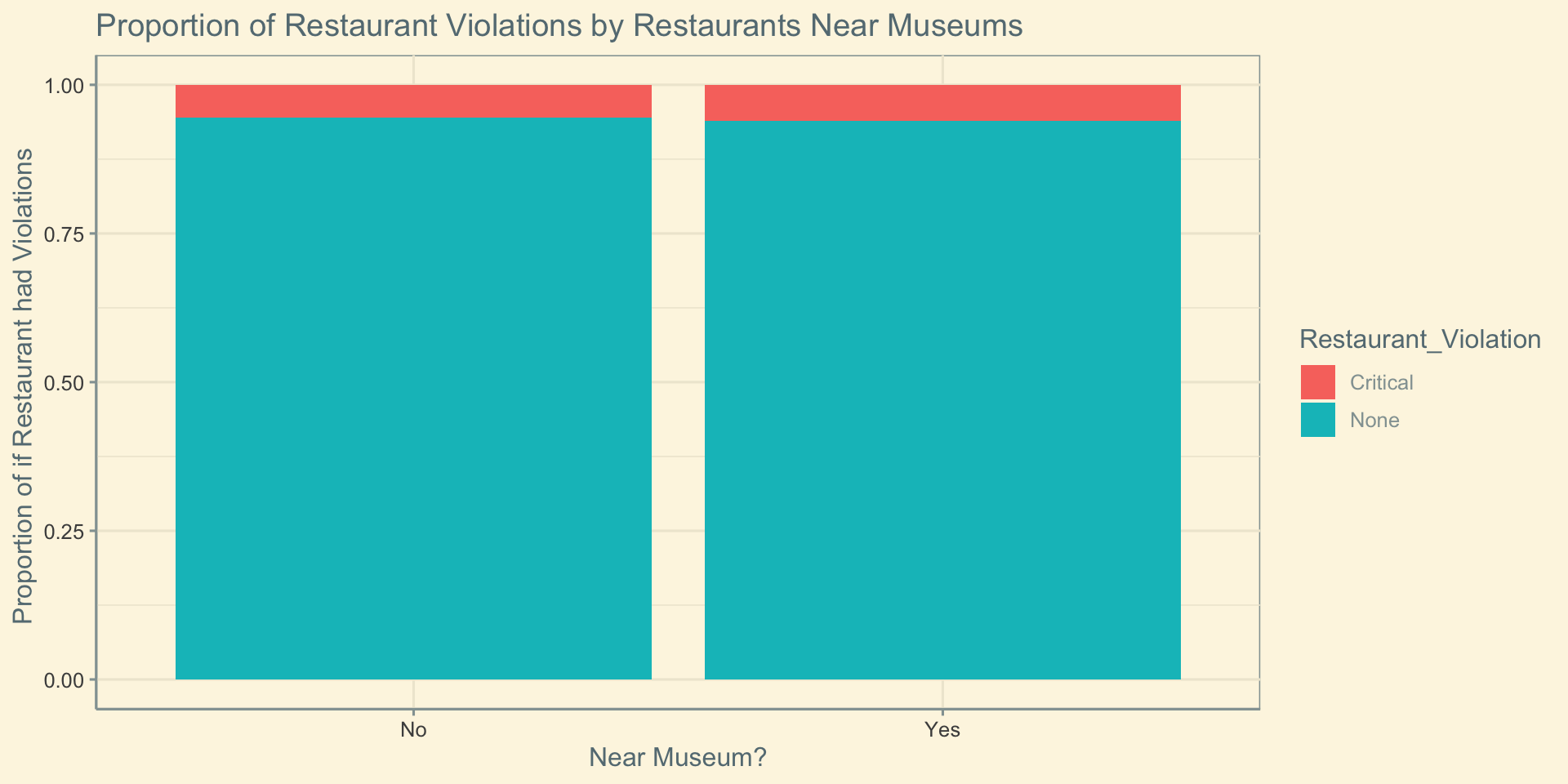
Goal 2: Visualizing the Analysis
We are visualizing the proportion of if a restaurant ever had violations (None, Critical) by if restaurants are near museums (yes,no).
![]()
Figure 6
Chi-Square Analysis for Goal 2
    Pearson's Chi-squared test with Yates' continuity correction

data:  contingency_table_2
X-squared = 1.4637e-28, df = 1, p-value = 1
                    Near_Museum
Restaurant_Violation        No       Yes
            Critical  30.38585  4.614148
            None     509.61415 77.385852
The chi-square test shows X^2 = 6.2237e-30, df = 2, p = 1
Cramer’s V tells us that the relationship is very weak in strength (0.008128).
Continuation
    Fisher's Exact Test for Count Data

data:  contingency_table_2
p-value = 0.7978
alternative hypothesis: true odds ratio is not equal to 1
95 percent confidence interval:
 0.3339362 3.0818476
sample estimates:
odds ratio
 0.9060068
- p value is 0.7975, which is still not a statistically significant relationship between restaurants being near museums and restaurant violations.
Goal 3: Creating an interactive Map
Key takeaway
- Red: Low Rated Restaurants
- Purple: Average Rated Restaurants Dark
- Blue: High Rated Restaurants.
- Black: Museums
Project Relevance to New Yorkers
I believe that this project is relevant to New Yorkers who like to go to museums or restaurants and would like to plan an outing for a nice museum day in NYC. These types of New Yorkers would care about this type of project because they no longer have to rely on using Google to search each individual museum and instead have a map that is accessible and easy to use.
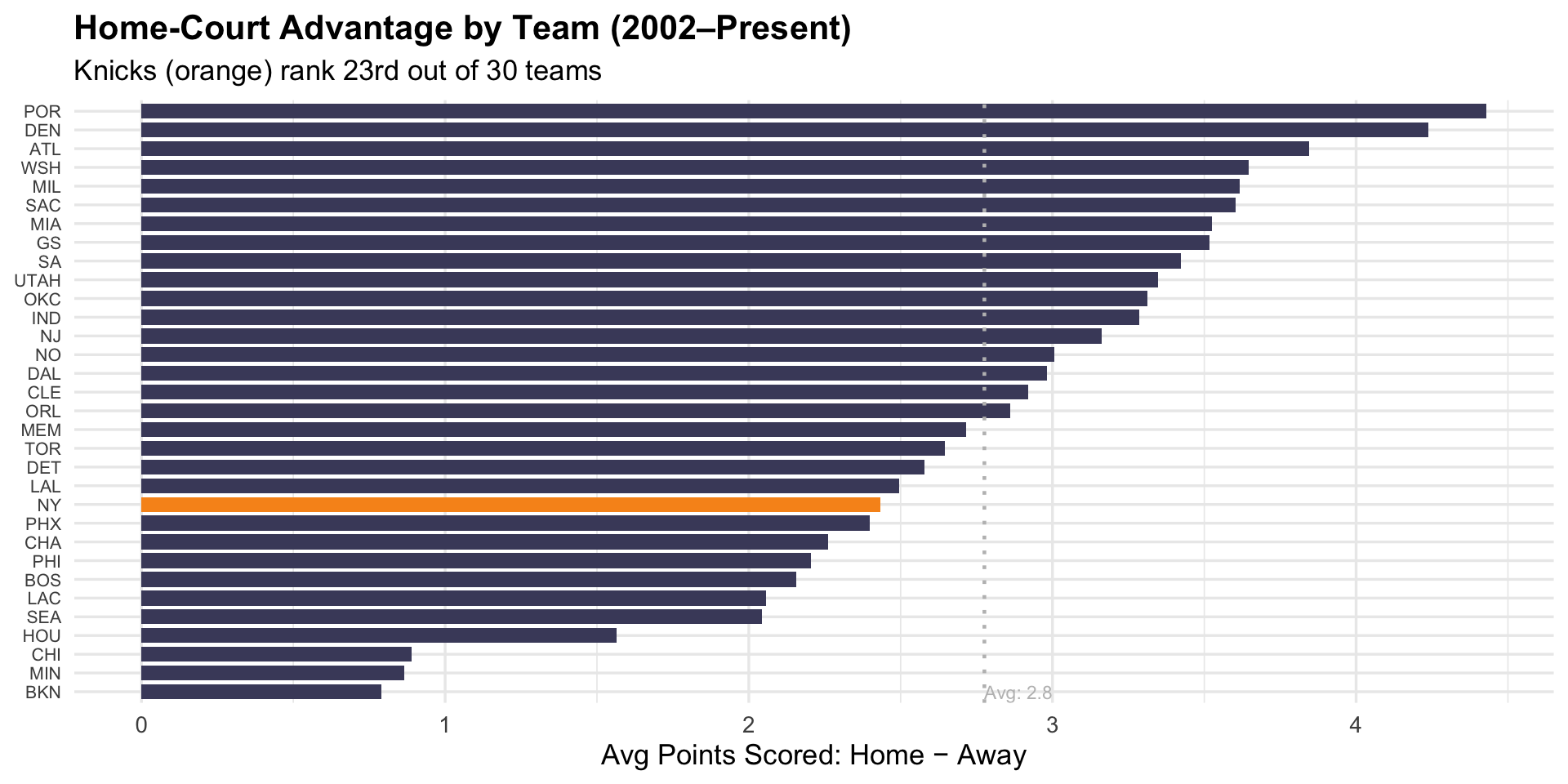
Background
- Oldest active NBA arena (est. February 11, 1968)
- Home-court of the New York Knicks, one of the league’s most valuable franchises
- NYC’s premier indoor venue comes with prestige and disproportionate national coverage
- Dozens of celebrities, athletes, public figures in attendance of every game
- Iconic performances: Jordan’s 55-pt return from retirement (1995), Kobe’s MSG record-setting 61-pt game (2009), Curry’s 54-pt 11/13 from three breakout game (2013)
Madison Square Garden, “The Mecca of Basketball”
The narrative: MSG uniquely influences players’ performances under its bright lights.
But is that narrative supported by data?
Research Questions
Q1: Do the Knicks experience a special home-court advantage at MSG compared to other NBA teams at their home arenas?
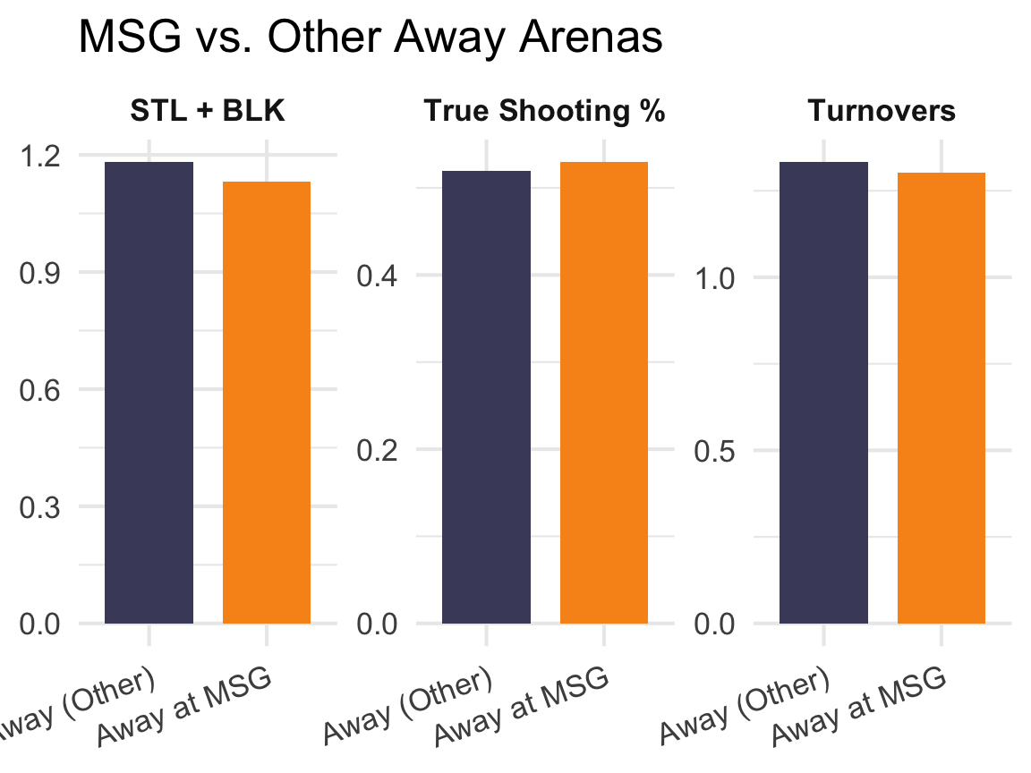
Q2: Do visiting players perform differently at MSG than at other away arenas?
Q3: Which players benefit most (or least) from playing at MSG?
Methods & Data
- Source:
hoopR R package: NBA game and player box score data, 2002–present
- Scope: Standard regular season and playoff games only
- Key metrics: Points, True Shooting % (TS%), Turnovers, Offensive Output (PTS + REB + AST), Defensive Output (STL + BLK)
- Player analyses excludes Knicks players home games; MSG data reflects visiting teams only
- Comparisons use independent samples t-tests
Q1: Knicks Home-Court Advantage
- The Knicks rank 23rd out of 32 teams in home-court scoring advantage
- Bottom 1/3 of the league.
- MSG as a home-court may actually be more of a detriment than a benefit.
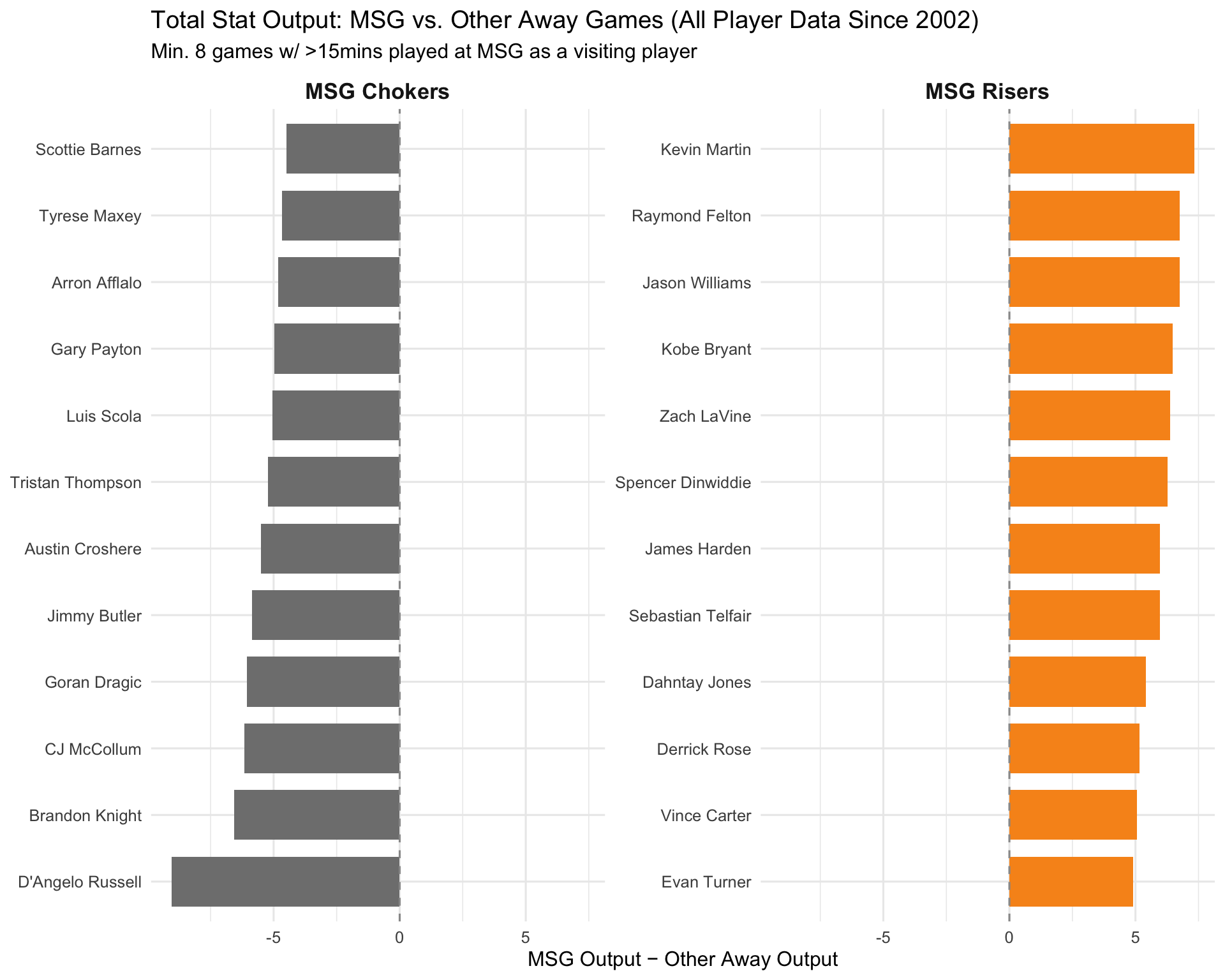
Q3: Who rises to the occasion at MSG? Who struggles?
The influence of playing at MSG on individual players’ statistical production depends on the player.
Knicks fans:
- Do the players on the left seem overrated by other NBA fans? Any NBA villains?
Conclusions
- Q1: The Knicks’ home-court advantage at MSG is actually worse than most NBA teams.
- Q2: Visiting players show small but statistically significant differences at MSG compared to other away arenas. On average, players shoot more efficiently and turn the ball over less, but produce less blocks and steals.
- Q3: There is meaningful individual variation in how players perform at MSG relative to their road averages.
- Takeaway: While players across the NBA perform better offensively at MSG, the “MSG effect” is not a homogeneous influence on players; some perform better and others worse when they play at MSG compared to other away arenas.
Isley Jean-Pierre
Examining How Juvenile Probation And School Discharge Contribute To Recidivism
Introduction
- Juvenile recidivism remains a major policy concern
- Probation supervision and school outcomes may influence rearrest rates
- This project investigates:
- Rearrest Rates, Probation Caseloads, and School Discharge Patterns
Goal: To help policymakers evaluate whether current probation resources are sufficient to reduce recidivism among youth.
Research Questions
How does supervision caseload relate to rearrest rates among youths?
What can school discharges tell us about supervision caseloads and rearrest rates?
Results
How does supervision caseload relate to rearrest rates among youths?
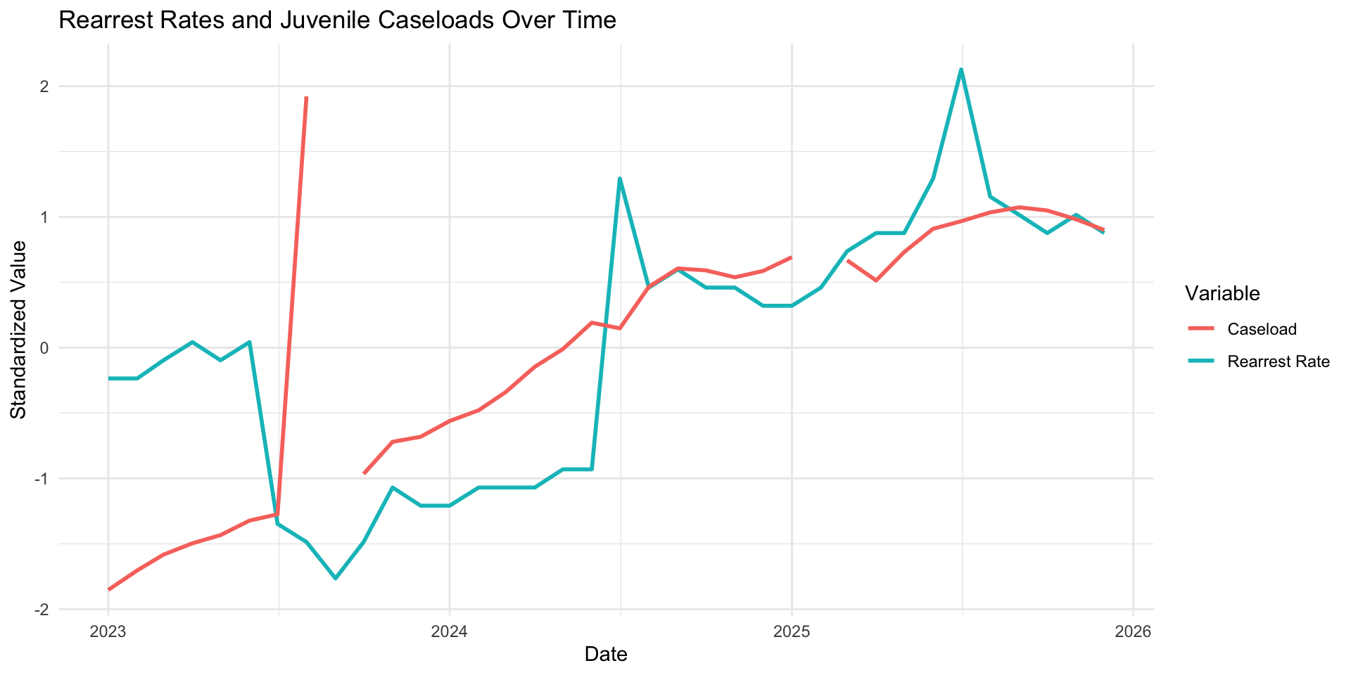
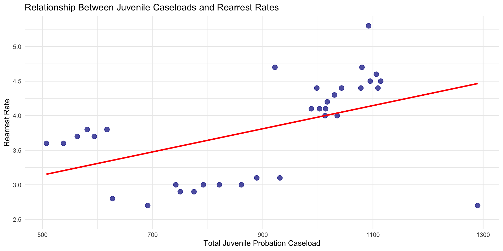
A correlation analysis (r = 0.49) shows a weak positive relationship between supervision caseloads and rearrest rates among the youths.
A regression analysis (p < .003) indicates that juvenile caseloads significantly predict rearrest rates. R-squared = 0.24 (24%).
Overall, these results signify that more caseloads tend to lead to more rearrest rates.
Time Series Analysis
![]()
Figure 10
Regression Analysis
![]()
Figure 11
Results
What can school discharges tell us about supervision caseloads and rearrest rates?
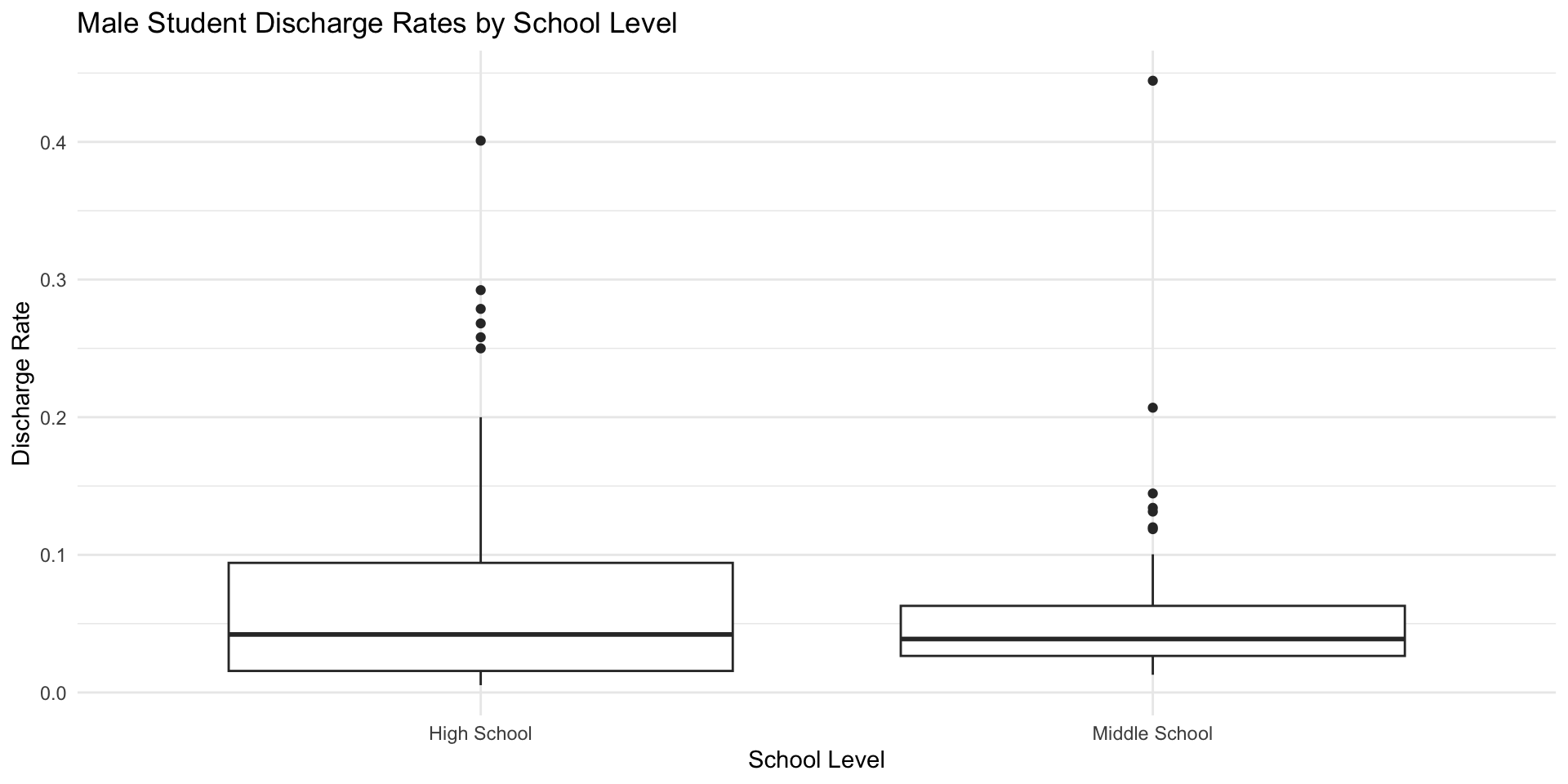
An independent t-test (t = 1.15, df = 159.43, p < 0.25) shows no significant difference between school discharge rate and school level.
A Chi-square analysis (X-squared = 938.62, df = 1, p < 2.2e-16) suggests a significant difference between discharge category and school level.
Cramer’s V (0.54). Moderate to strong relationship between discharge category and school level.
    Welch Two Sample t-test

data:  discharge_rate by school_level
t = 1.1492, df = 159.43, p-value = 0.2522
alternative hypothesis: true difference in means between group High School and group Middle School is not equal to 0
95 percent confidence interval:
 -0.008913023  0.033721970
sample estimates:
  mean in group High School mean in group Middle School
                 0.06976680                  0.05736233
    Wilcoxon rank sum test with continuity correction

data:  discharge_rate by school_level
W = 3034, p-value = 0.381
alternative hypothesis: true location shift is not equal to 0
Discharge Rates By School Level
![]()
Figure 12
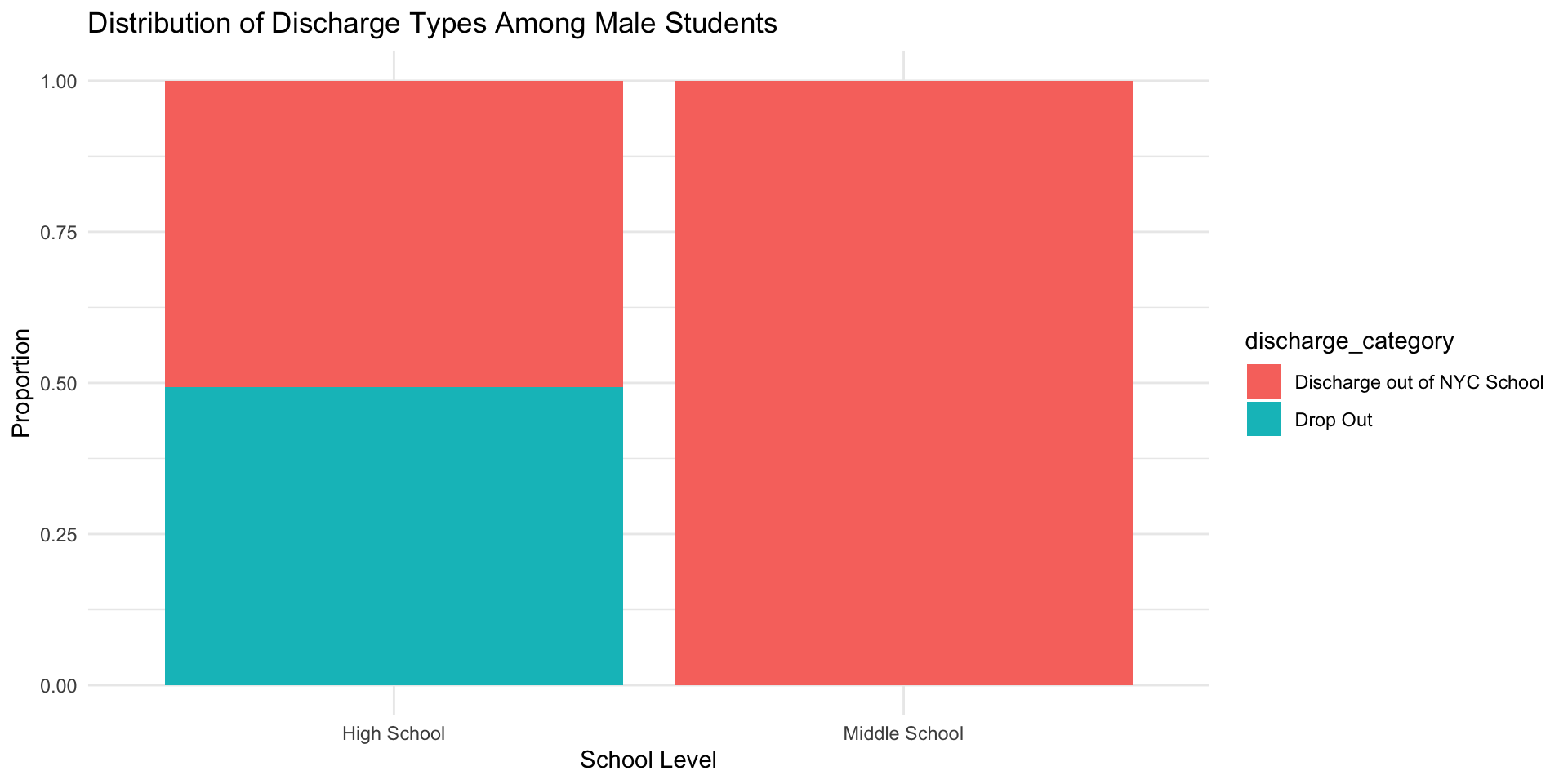
Discharge Types By School Level
![]()
Figure 13
School Discharges By Districts
Conclusion
- Caseload size is significantly related to rearrest rates
- School discharge patterns differ by school level
- Too many caseloads may reduce supervision effectiveness
- Education disruptions can potentially lead to crime involvement
- Demographic variables
Shannon Joyce
Toxic Homes: Exploring Mold Exposure Complaint and Domestic Violence Report Trends in NYC
Project Overview
Do domestic violence reports and residential mold complaints in NYC follow similar, correlated patterns over time?
Datasets: Mold Complaints
311 Service Requests
Table 1. Aggregated residential mold complaints by borough, 2010-2024.
| 2010 |
01 - January |
BRONX |
954 |
| 2010 |
01 - January |
BROOKLYN |
779 |
| 2010 |
01 - January |
MANHATTAN |
410 |
| 2010 |
01 - January |
QUEENS |
315 |
| 2010 |
01 - January |
STATEN ISLAND |
58 |
Datasets: Domestic Violence Reports
NYPD Complaint Data Historic
Table 2. Aggregated domestic violence reports by borough, 2010-2024.
| 2010 |
01 - January |
BRONX |
910 |
| 2010 |
01 - January |
BROOKLYN |
1306 |
| 2010 |
01 - January |
MANHATTAN |
541 |
| 2010 |
01 - January |
QUEENS |
791 |
| 2010 |
01 - January |
STATEN ISLAND |
154 |
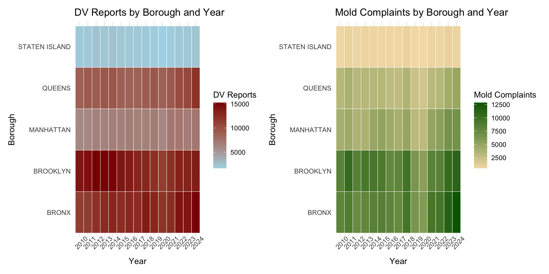
Exploratory Analysis: Heat Maps
![]()
Figure 1. DV reports & mold complaints by borough and year, 2010-2024. Darker colors represent a higher volume of complaints/reports.
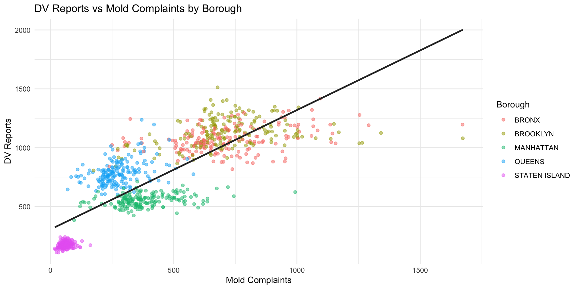
Correlation Plot: Totals by Borough
![]()
Figure 2. A scatterplot representing a positive correlation between total mold complaints and DV reports, grouped by borough.
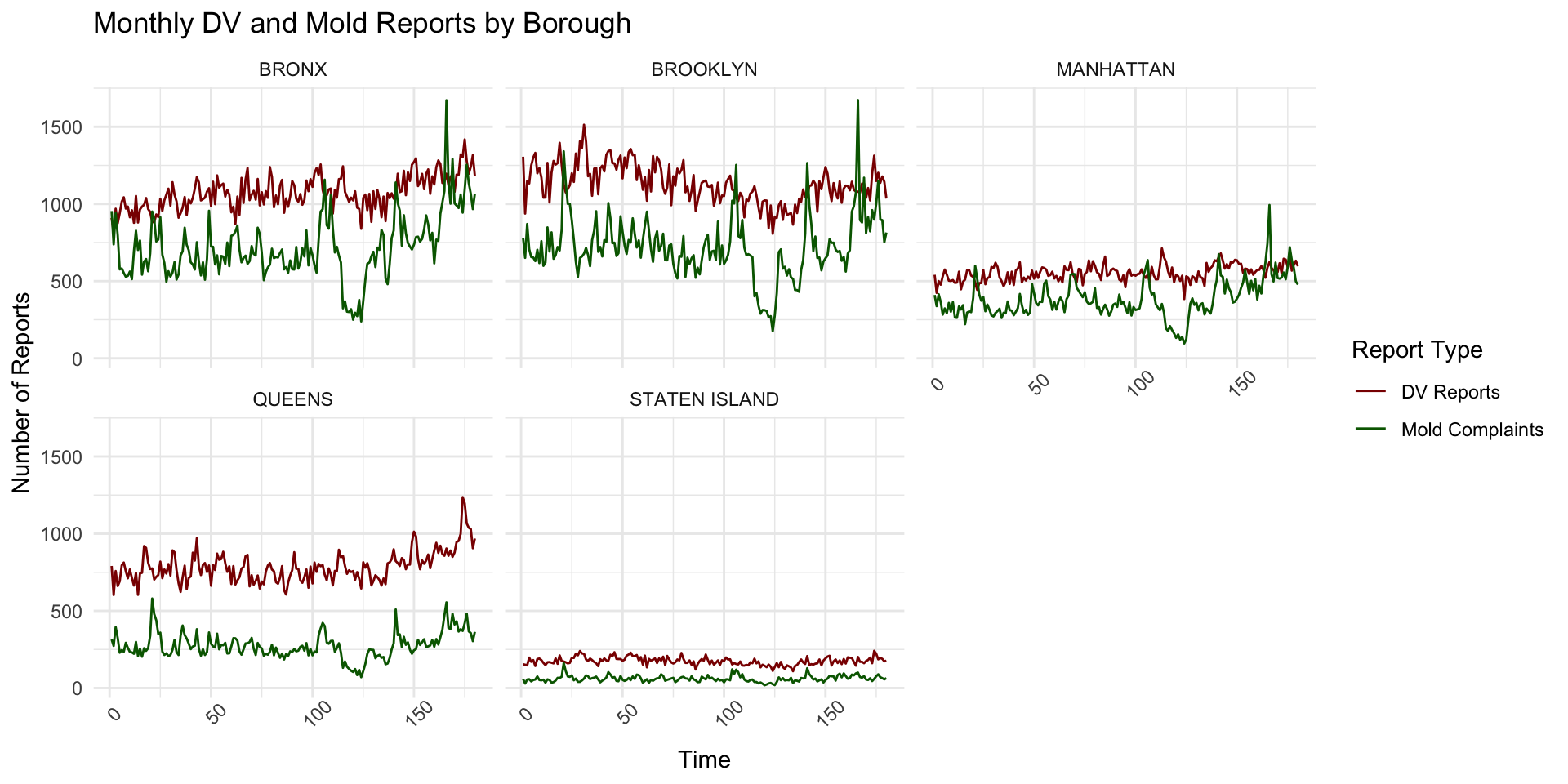
Exploratory Analysis: Temporal Trends by Borough
![]()
Figure 3. Line plots representing monthly DV reports & mold complaints by borough, 2010-2024.
Correlation Test: DV Reports ~ Mold Complaints (Month to Month)
    Pearson's product-moment correlation

data:  x and y
t = 5.1733, df = 178, p-value = 6.155e-07
alternative hypothesis: true correlation is not equal to 0
95 percent confidence interval:
 0.2272817 0.4822876
sample estimates:
      cor
0.3615268
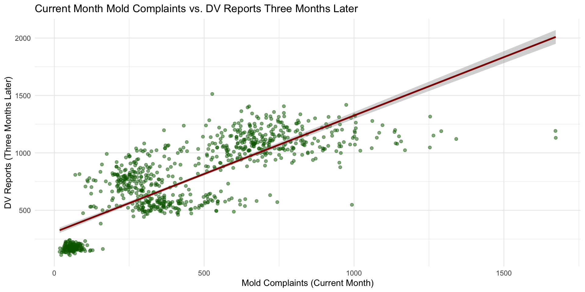
Correlation Plot: Lagged Data
![]()
Figure 4. A scatterplot representing a positive correlation between current-month mold complaints and DV reports 3 months later.
Correlation Test: Lagged Data
Current Month Mold Complaints ~ DV Reports 3 Months Later
Regression Models
| Mold ~ DV + Borough |
0.94 |
< 0.001 |
10571.03 |
| Mold ~ DV + Borough + Avg. Resolution Days |
0.95 |
< 0.001 |
10524.65 |
| Mold ~ DV (3 Months Later) + Borough |
0.94 |
< 0.001 |
10390.65 |
Key Findings & Takeaways
- Housing distress 🔗 Domestic instability
- Predictive power of both models
- Response speed
- 3-month lag
- Proactive roadmap for NYC agencies
- NYC Housing Authority
- NYC Department of Health & Mental Hygiene
Full Project: https://rpubs.com/shannonjoyce/toxichomes
Emma Valentina Tupone
Environmental Stressors and Social Complaints in NYC
Project Overview
Climate change increases urban environmental stress
Flooding can disrupt infrastructure and communities
Social stress may appear in complaint behavior
Research Question
- Do flooding complaints relate to noise complaints across NYC boroughs?
Data Preview
flooding
noise
Exploratory Summary
Flood complaints vary across boroughs and years
Noise complaints show even larger variation
Some boroughs report very high complaint activity
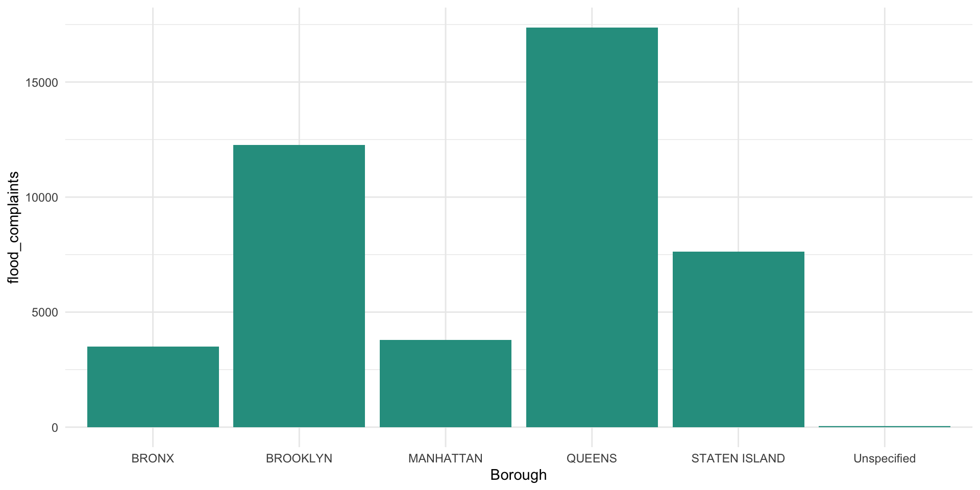
Flooding Complaints by Borough
![]()
Figure 14
Visual comparison of flooding complaints
Shows variation across boroughs
Highlights environmental vulnerability differences
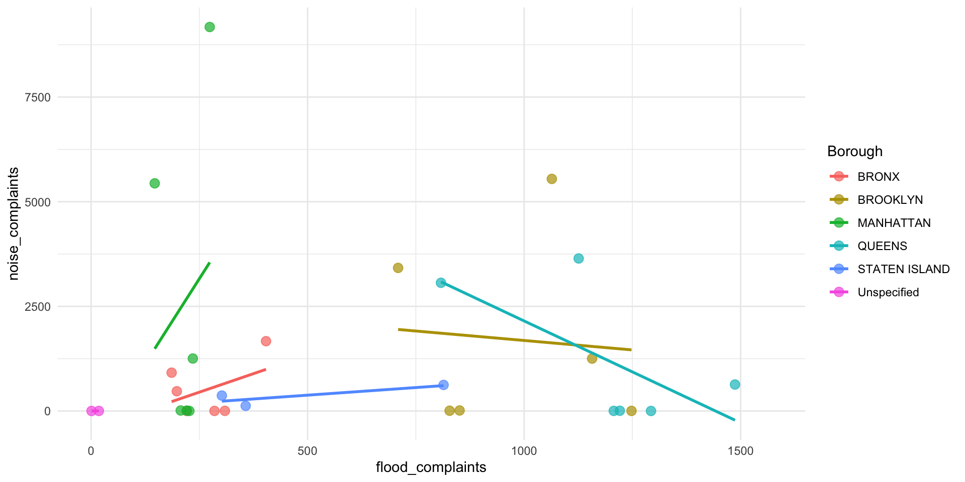
Correlation
![]()
Figure 15
Key Takeaways
Flood complaints vary across NYC boroughs
Noise complaints vary widely
Relationship between the two was weak
Environmental stress likely influenced by multiple factors
NYC Open Data enables civic research
Xinru Wang
Beating Around the Bush: Urban Trees and Wildlife Patterns in New York City
Urban Wildlife in NYC
Wildlife incidents are reported across NYC every day.
But they are not evenly distributed across boroughs.
What explains these patterns?
Could Street Trees Influence Wildlife Incidents?
At first glance, this might seem unlikely. Street trees line sidewalks, while many wildlife incidents occur in parks. But urban ecosystems are connected.
Street trees can support urban wildlife by providing:
• Food
• Shelter
• Travel pathways
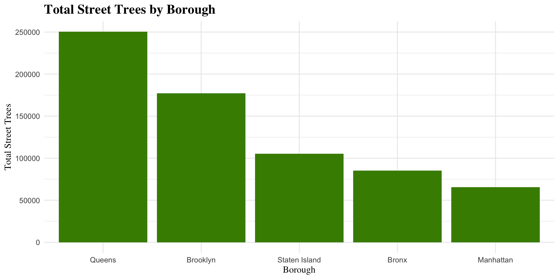
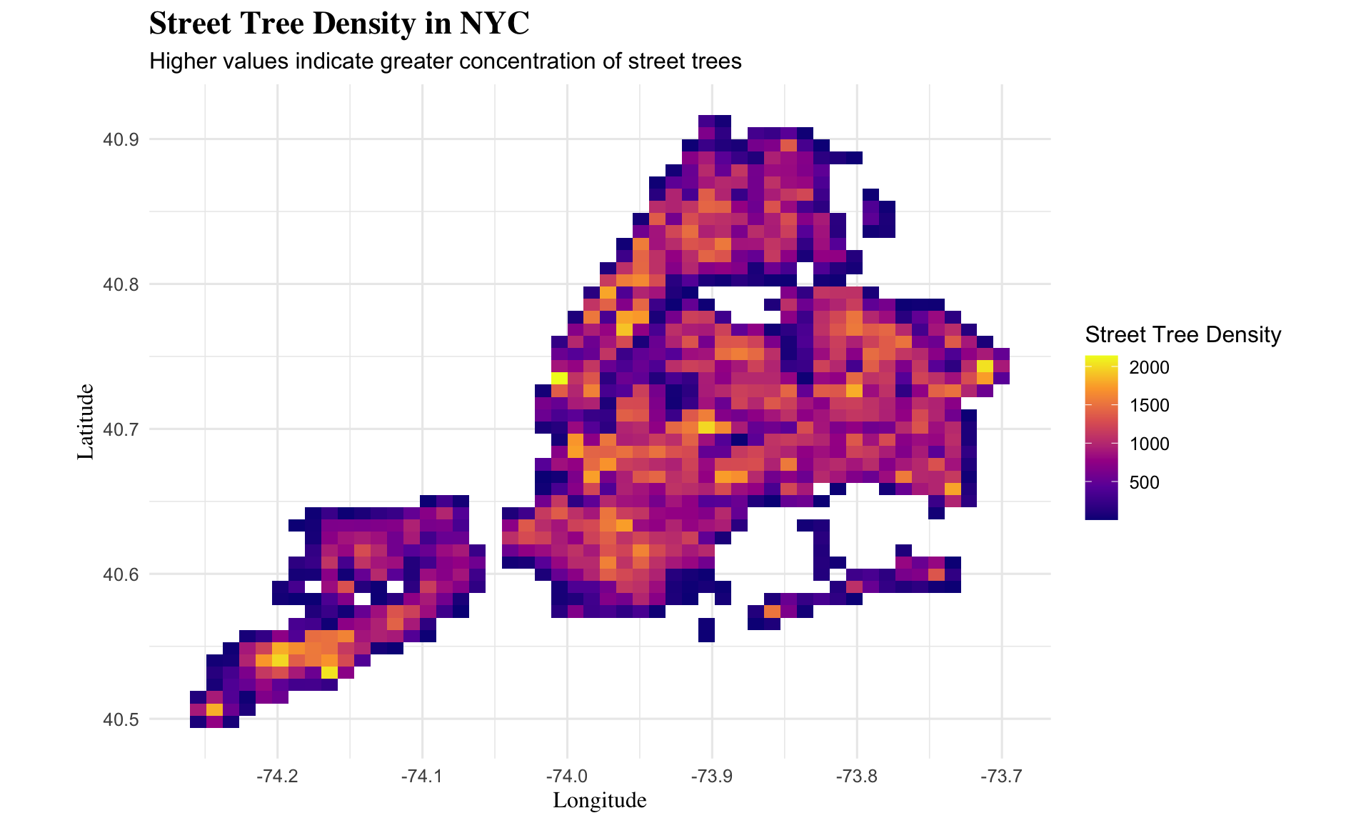
2015 NYC Street Tree Census
• Over 680,000 street trees recorded across NYC
• Includes species, location, and health condition
• Used to estimate urban canopy coverage
![]()
Figure 16
Urban Park Ranger Wildlife Incident Reports
- Reports of wildlife incidents across NYC parks
- Includes injured animals, distressed wildlife, and conflicts with humans
- Allows us to track wildlife activity patterns
![]()
Figure 17
Street Tree Density Across New York City
![]()
Figure 18: Brighter colors indicate higher concentrations of street trees.
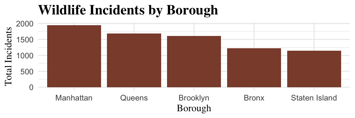
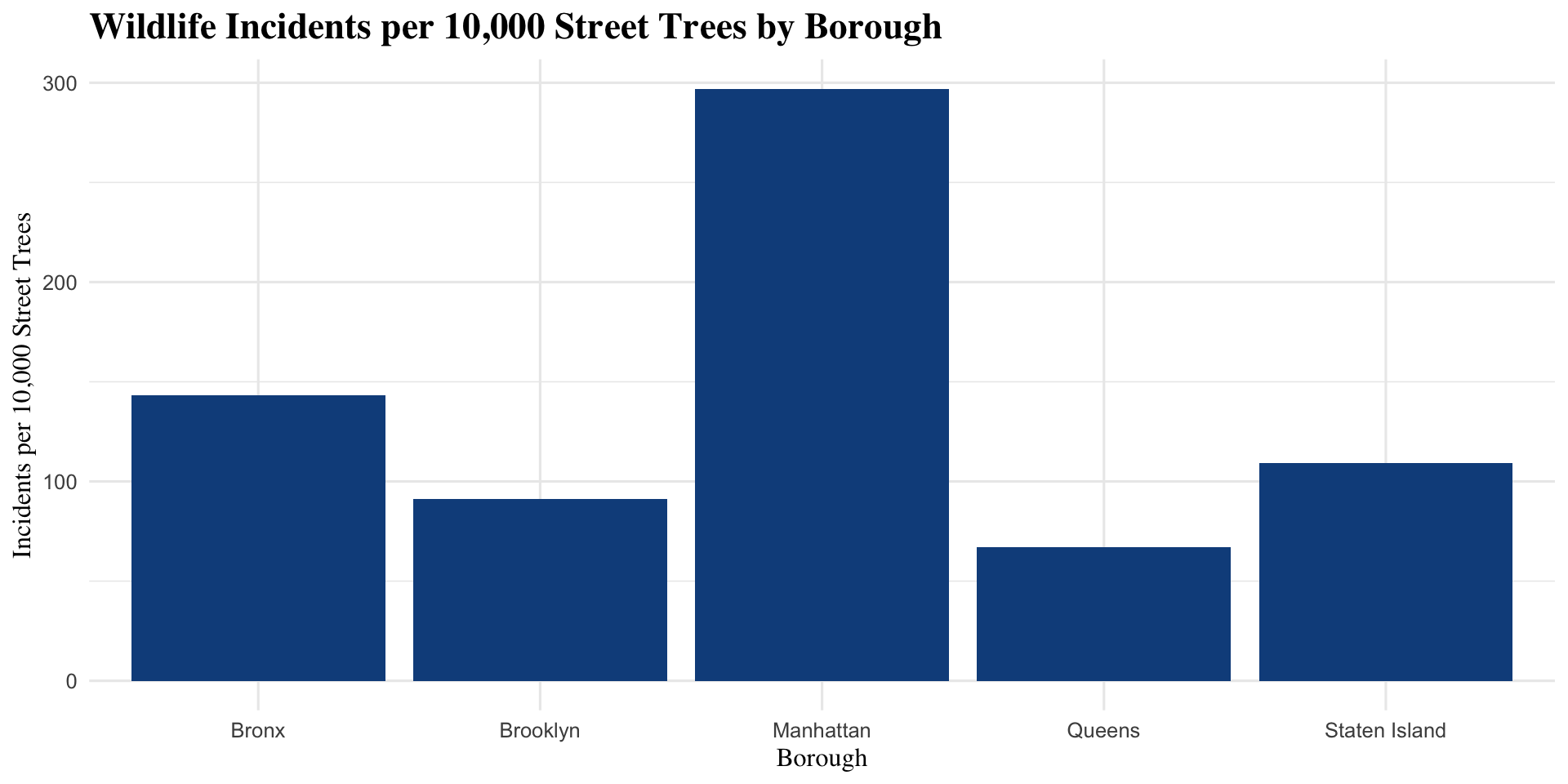
Wildlife Incidents per 10,000 Street Trees
![]()
Figure 19: How many wildlife incidents occur for every 10,000 street trees.
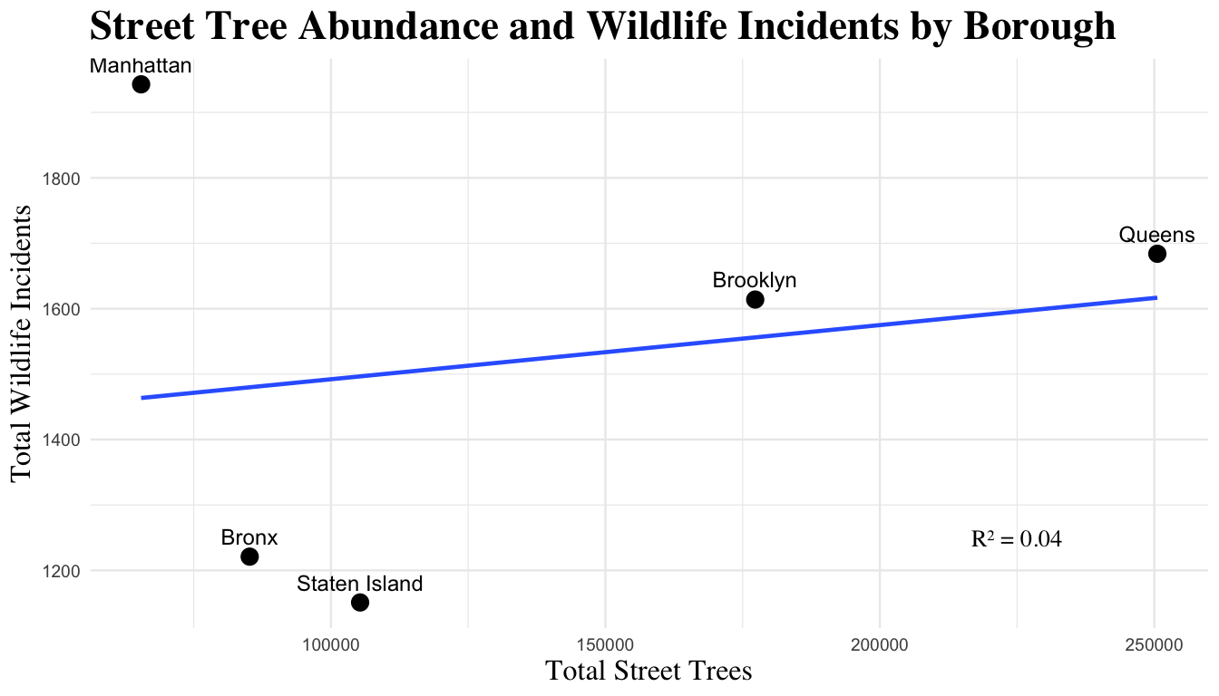
Weak Relationship Between Street Trees and Wildlife Incidents
![]()
Figure 20: Each point represents a NYC borough.
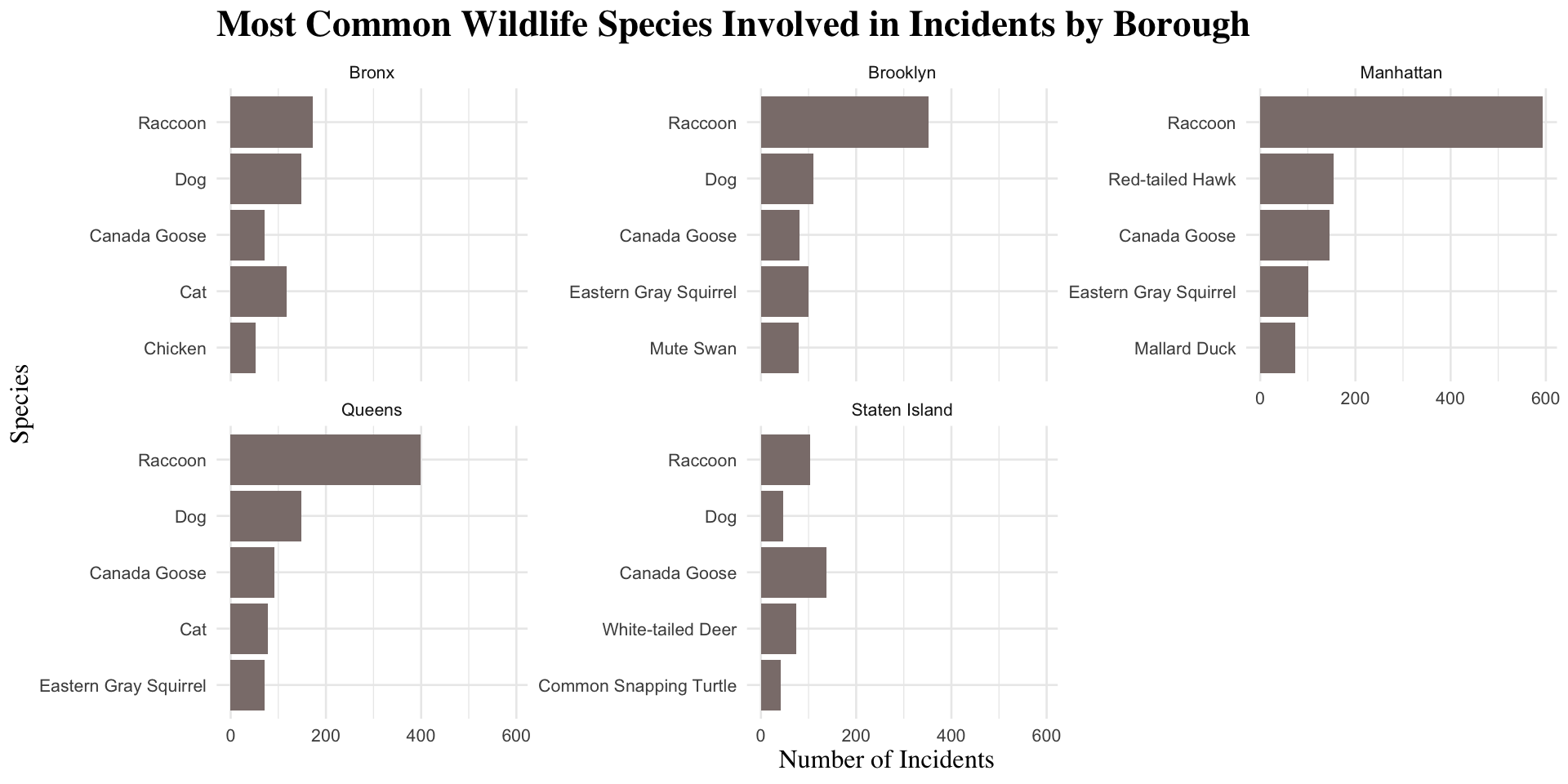
Raccoons Dominate Wildlife Incidents Across NYC
![]()
Figure 21: Raccoons appear most frequently in wildlife incident reports across boroughs.
Key Takeaways
Street tree abundance alone does not strongly predict wildlife incidents
Wildlife incidents vary across boroughs
Raccoon are the most commonly reported species
Other urban factors likely drive wildlife encounters
Laura Werner
Domestic Violence Incidents vs Resource Allocation Across NYC
Research Question
Are domestic violence resources for victims meeting the needs of victims in New York City?
This project compares reported domestic violence incidents with Family Justice Center (FJC) service utilization.
The analysis focuses on 2020 so that incidents and service usage are directly comparable.
The goal is to determine whether boroughs with greater reported need also show stronger support service engagement.
Why This Matters
Domestic violence is a major public safety and public health issue.
Harm extends beyond immediate injury and includes long-term emotional, psychological, and developmental consequences.
Children exposed to violence in the home may also experience lasting effects.
Timely and effective support services are critical for survivor safety, recovery, and prevention of future harm.
Data Sources via NYC Open Data
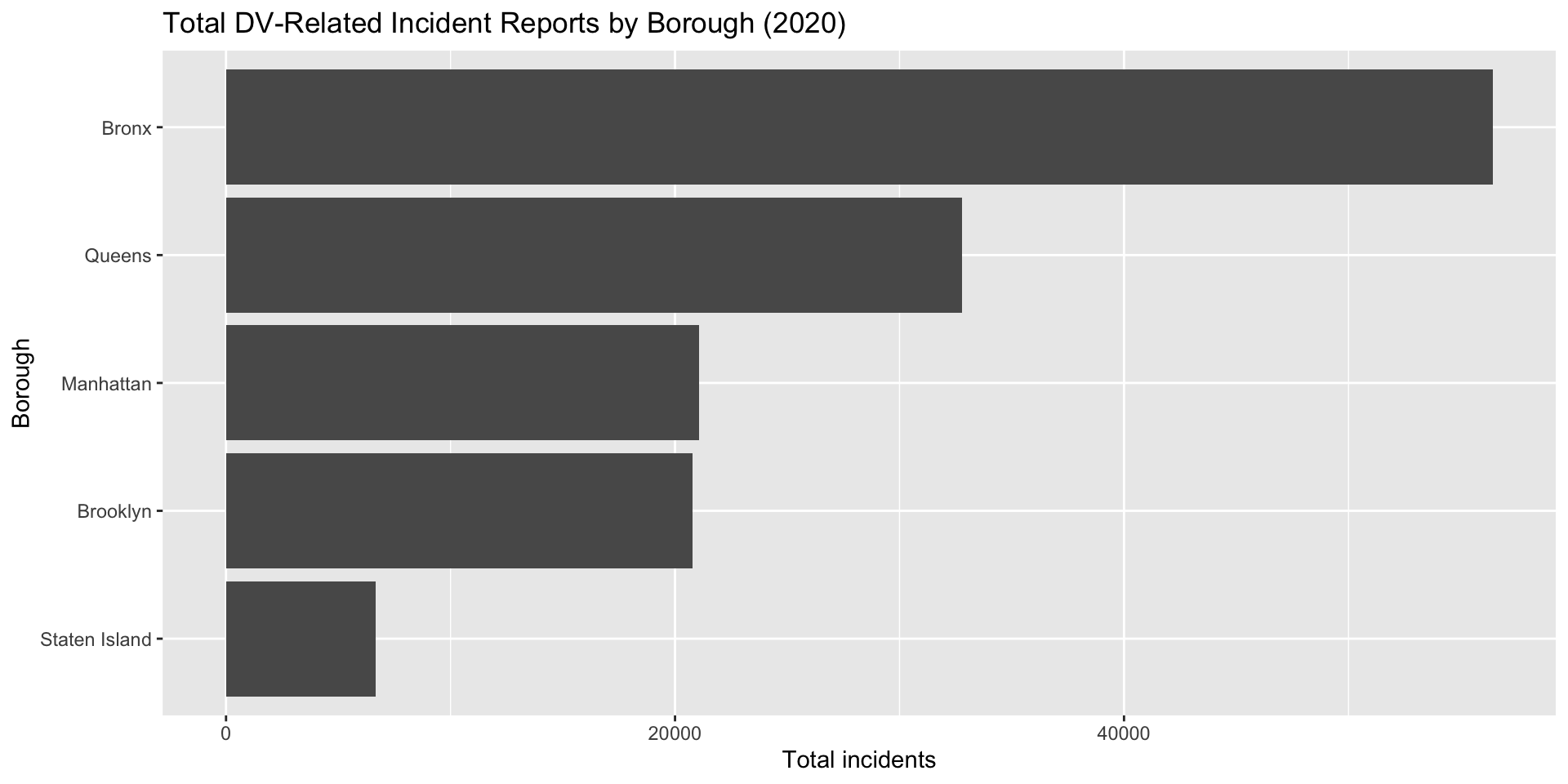
Key Interpretation
The Bronx had the highest total number of reported domestic violence–related incidents.
Queens followed next.
Manhattan and Brooklyn showed similar moderate levels.
Staten Island had the fewest reported incidents.
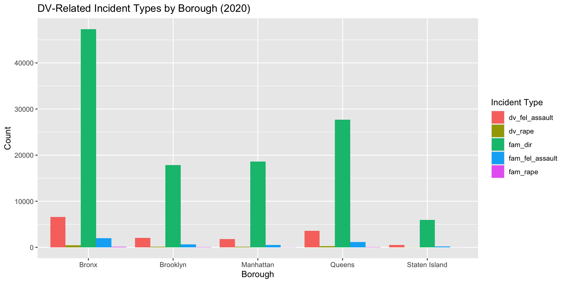
Incident Type by Borough
![]()
Figure 23
Key Interpretation
Family domestic incident reports dominate across all boroughs.
Felony assaults and rape-related offenses occur at much lower frequencies.
The Bronx remains consistently high across most incident categories.
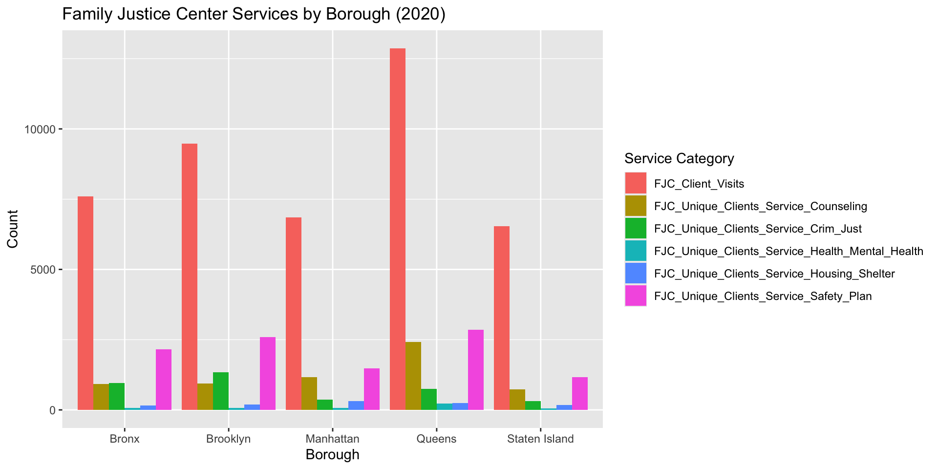
Family Justice Center Services by Borough
![]()
Figure 24
Key Interpretation
Family Justice Center client visits are much higher than services being provided.
Queens shows the highest overall service utilization.
Manhattan and Staten Island show lower totals across many categories.
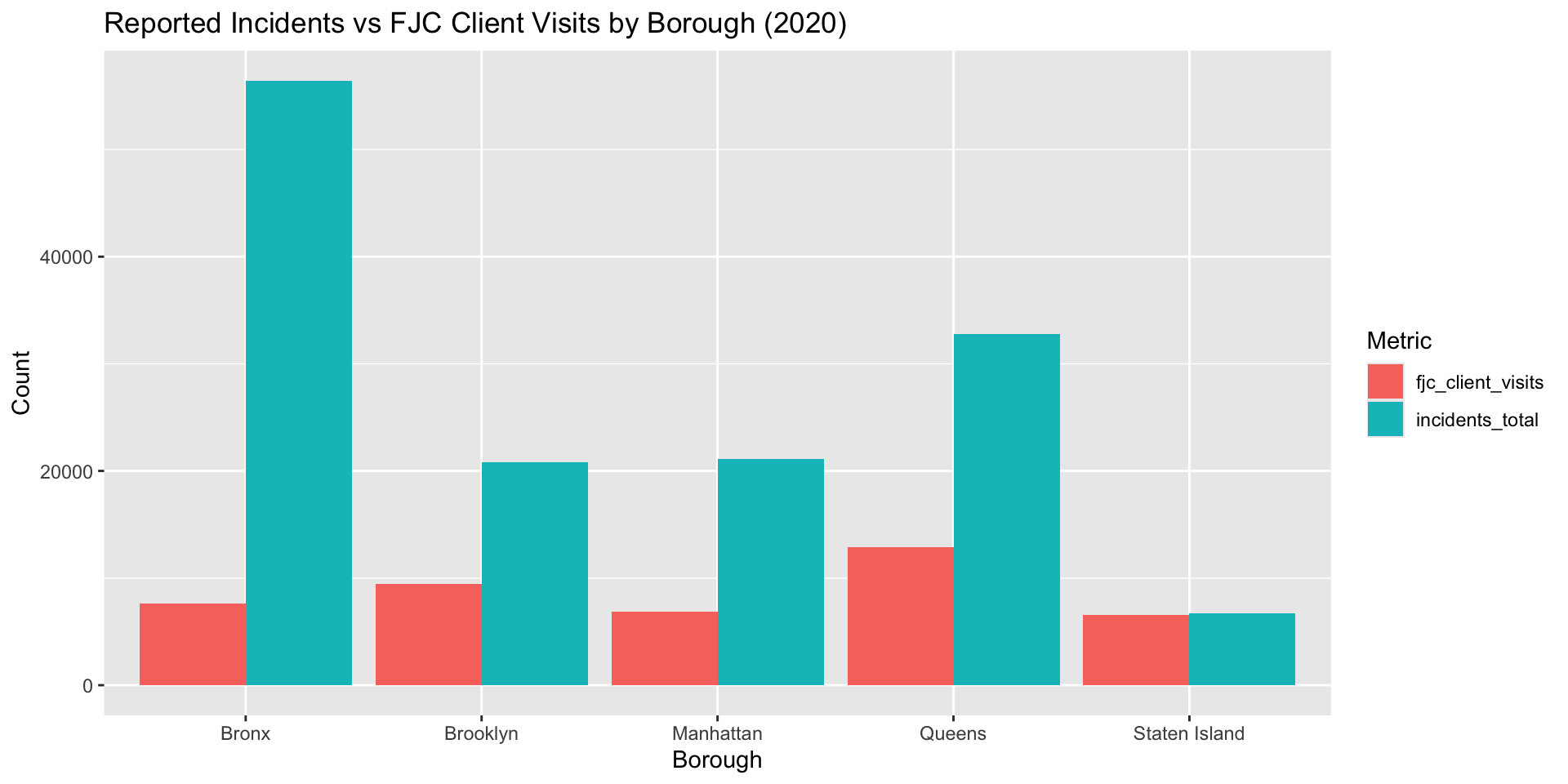
Comparing Incidents and Client Visits
![]()
Figure 25
Key Interpretation
Boroughs with more reported incidents generally have more client visits.
However, the relationship is not proportional.
The Bronx has the highest incident burden but not the highest number of FJC client visits.
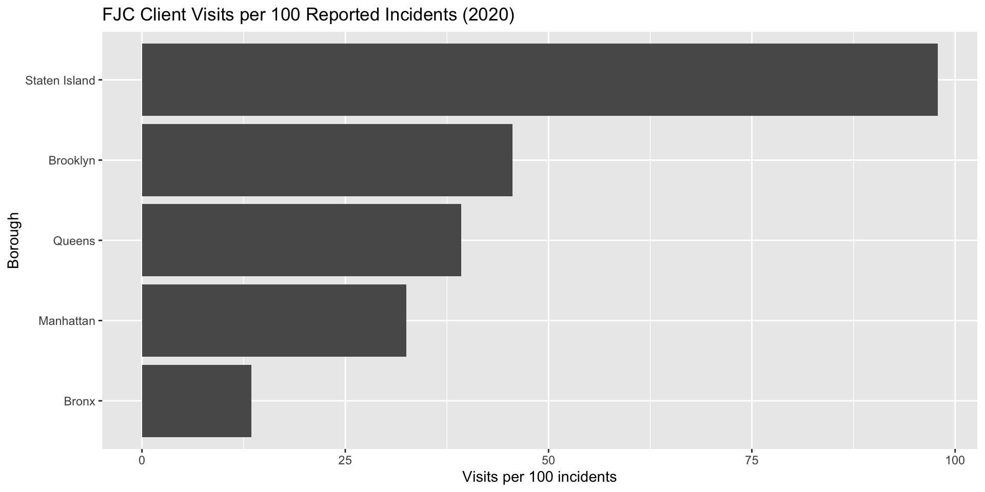
FJC Client Visits per 100 Reported Incidents
![]()
Figure 26
Key Interpretation
Standardizing visits by incident burden reveals sharper disparities.
Staten Island has the highest visits per 100 incidents.
The Bronx has the lowest.
This suggests that high-need boroughs may not be receiving equally accessible support.
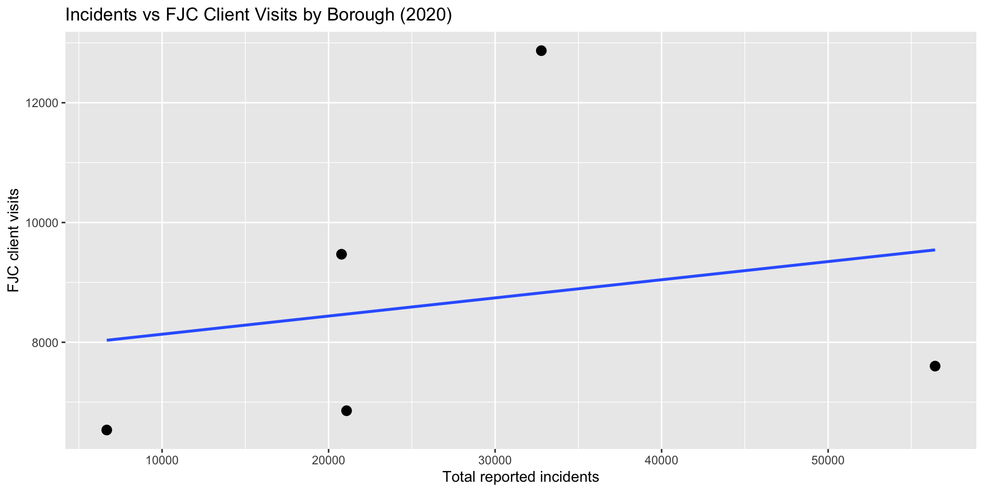
Scatterplot: Incidents vs Client Visits
![]()
Figure 27
Key Interpretation
The pattern suggests a weak positive relationship.
Still, boroughs vary noticeably around the trend line.
Service engagement does not rise proportionally with domestic violence burden.
Discussion
Domestic violence resources are not evenly aligned with reported need across NYC boroughs. The Bronx shows the highest incident burden but the lowest service engagement relative to need.Staten Island shows much higher service engagement per reported incident. These disparities may reflect:
Conclusion
The findings raise concerns about whether domestic violence resources are adequately meeting survivor needs across NYC.
In the highest-need boroughs, especially the Bronx, service engagement appears disproportionately low.
This is not just a statistical gap, but moreover it reflects real consequences for survivor safety, well-being, and long-term stability.
Improving access, visibility, and distribution of services is a public responsibility.
Final Takeaway
Higher reported need does not always correspond to stronger service engagement.
To better support survivors, NYC should evaluate how domestic violence services are distributed, promoted, accessed and resourced across boroughs.