Analyzing NYC Climate Projections: Extreme Events and Sea Level Rise
Emma Tupone
Source:vignettes/analyzing-nyc_events_sealevel.Rmd
analyzing-nyc_events_sealevel.RmdIntroduction
This vignette demonstrates how to use the 38ps-fnsg() function to explore projected extreme climate events and sea level rise for New York City using the New York City Climate Projections: Extreme Events and Sea Level Rise dataset on the NYC Open Data portal.
The dataset provides projections under different climate scenarios, including:
- Number of heatwaves per year
- Cooling and heating degree days
- Projected sea level rise
Researchers, city planners, and policymakers can use this information to understand future climate risks, prepare for extreme weather events, and plan adaptation strategies.
Retrieve a Sample of Data
sample_data <- nyc_pull_dataset("38ps-fnsg", limit = 10)
nyc_list_datasets()
#> # A tibble: 2,389 × 26
#> key uid name datasetinformation_a…¹ description type category
#> <chr> <chr> <chr> <chr> <chr> <chr> <chr>
#> 1 orr_points dhcf… ORR_… Mayor's Office of Cli… "Completed… data… City Go…
#> 2 off_year_and_s… ups9… Off-… Campaign Finance Boar… "This data… data… City Go…
#> 3 parks_trails vjbm… Park… Department of Parks a… "Location … data… Environ…
#> 4 where_the_doll… qhm5… Wher… Mayor's Office of Man… "This data… data… City Go…
#> 5 citywide_mobil… rb38… City… Department of Transpo… "In 2020, … data… Transpo…
#> 6 x2013_2014_sch… ac4n… 2013… Department of Educati… "School Lo… data… Educati…
#> 7 tourism_grants rma9… Tour… Brooklyn Borough Pres… "Final lis… data… City Go…
#> 8 citywide_cash_… 9jbx… City… Human Resources Admin… "Total num… data… Social …
#> 9 nyc_domain_reg… ymvu… .nyc… Office of Technology … ".nyc doma… data… Business
#> 10 nycha_developm… evjd… NYCH… New York City Housing… "Contains … data… Housing…
#> # ℹ 2,379 more rows
#> # ℹ abbreviated name: ¹datasetinformation_agency
#> # ℹ 19 more variables: legislativecompliance_datasetfromtheopendataplan <chr>,
#> # url <chr>, update_datemadepublic <chr>, update_updatefrequency <chr>,
#> # last_data_updated_date <chr>,
#> # legislativecompliance_candatasetfeasiblybeautomated <chr>,
#> # update_automation <chr>, legislativecompliance_hasdatadictionary <chr>, …
sample_data
#> # A tibble: 10 × 16
#> period sea_lelel_rise number_of_days_year_…¹ number_of_days_year_…²
#> <chr> <chr> <dbl> <dbl>
#> 1 Baseline (1981-… n/a 69 17
#> 2 2030s (10th Per… 6 in 85 27
#> 3 2030s (25th Per… 7 in 85 27
#> 4 2030s (75th Per… 11 in 99 46
#> 5 2030s (90th Per… 13 in 104 54
#> 6 2050s (10th Per… 12 in 91 32
#> 7 2050s (25th Per… 14 in 99 38
#> 8 2050s (75th Per… 19 in 100 62
#> 9 2050s (90th Per… 23 in 121 69
#> 10 2080s (10th Per… 21 in 104 46
#> # ℹ abbreviated names: ¹number_of_days_year_with, ²number_of_days_year_with_1
#> # ℹ 12 more variables: number_of_days_year_with_2 <dbl>,
#> # number_of_days_year_with_3 <dbl>, number_of_heatwaves_year <dbl>,
#> # average_lenth_of_heat_waves <dbl>, number_of_days_year_with_4 <dbl>,
#> # number_of_days_year_with_5 <dbl>, cooling_degree_days <dbl>,
#> # number_of_days_year_with_6 <dbl>, heating_degree_days <dbl>,
#> # number_of_days_year_with_7 <dbl>, number_of_days_year_with_8 <dbl>, …This code retrieves 10 rows of data from the NYC Open Data endpoint for extreme events and sea level rise projections.
Summarize Key Metrics
summary_table <- sample_data |>
select(period, number_of_heatwaves_year, cooling_degree_days, heating_degree_days) |> dplyr::slice_head(n = 10)
summary_table
#> # A tibble: 10 × 4
#> period number_of_heatwaves_…¹ cooling_degree_days heating_degree_days
#> <chr> <dbl> <dbl> <dbl>
#> 1 Baseline (198… 2 1156 4659
#> 2 2030s (10th P… 3 1397 3589
#> 3 2030s (25th P… 3 1471 3766
#> 4 2030s (75th P… 6 1757 4049
#> 5 2030s (90th P… 7 1903 4240
#> 6 2050s (10th P… 4 1568 3102
#> 7 2050s (25th P… 5 1713 3384
#> 8 2050s (75th P… 8 2124 3754
#> 9 2050s (90th P… 9 2335 3996
#> 10 2080s (10th P… 6 1817 2298
#> # ℹ abbreviated name: ¹number_of_heatwaves_year- Period=climate period (e.g., “Baseline”, “2030s”)
- number_of_heatwaves_year=projected heatwaves per year
- cooling_degree_days/heating_degree_days=metrics of temperature extremes
This table gives a quick overview of projected extreme events for different scenarios.
Visualization
plot_data <- sample_data |>
  mutate(number_of_heatwaves_year = as.numeric(number_of_heatwaves_year))

ggplot(plot_data, aes(x = period, y = number_of_heatwaves_year)) +
  geom_col() +
  labs(
    title = "Projected Number of Heatwaves by Climate Period",
    x = "Climate Period",
    y = "Projected Heatwaves per Year"
  ) +
  theme_minimal() +
  theme(axis.text.x = element_text(angle = 45, hjust = 1))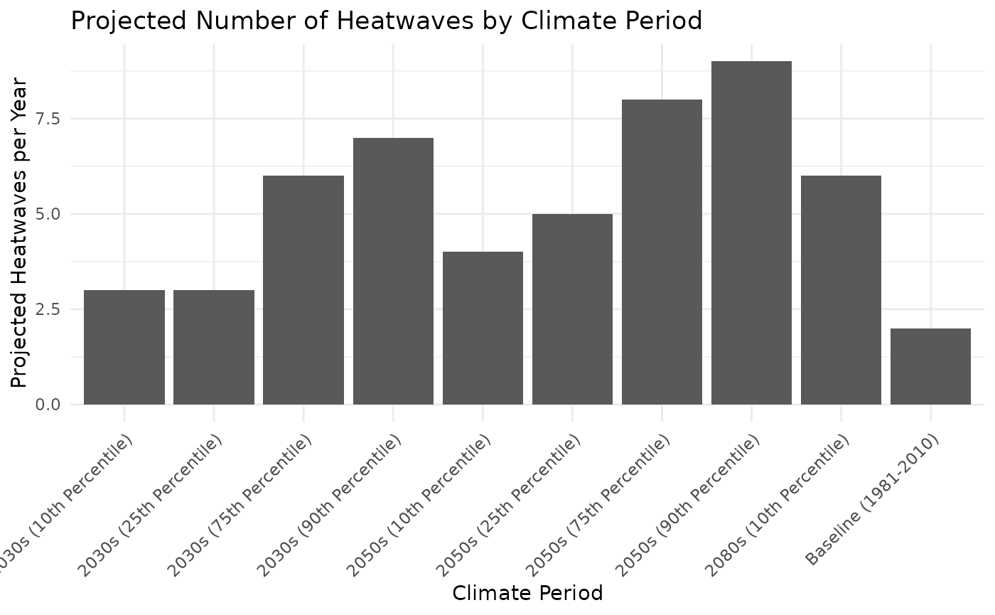
This plot shows how the number of heatwaves is projected to change across scenarios. It helps visualize future climate risks at a glance.